Realistic fluid simulations is an ever expanding and improving field in computer graphics. Several previous groups have attempted to tackle this topic and ended up creating water simulations that are physically accurate, but look more akin to jello. We are interested in creating a more realistic fluid simulation by also implementing water-air interactions like bubbles, spray, and foam. To do so, we implemented Position Based Fluids by Macklin and Müller for the underlying fluid simulation and Unified Spray, Foam and Bubbles for Particle-Based Fluids by Ihmsen et al. to simulate water-air interactions. To convert our fluid and water-air particles into a mesh we implemented the marching cubes algorithm using isotropic kernels. Finally we rendered the mesh using Blender's “Cycles” path tracing engine.
To implement our project, we started with a particle based water simulation.
Our code has a Fluid struct, which handles all of the Particle structs.
Each Particle struct has a list of their neighbors along with the current and previous position and velocity.
We use Euler's method along with incompressibility, collision, viscosity and vorticity constraints to update our Particle positions at each time step.
The incompressibility constraint applies a small change in position \(\Delta \textbf{p}_i\) to keep the volume of the fluid constant.
We estimate the density of each particle as \(\rho_i = \sum_j m_j W_{poly6} (\textbf{p}_i-\textbf{p}_j, \ h)\), where
\(W_{poly6} (\|\pmb{r}\|, h) = \begin{cases} (h^2 - \|\pmb{r}\|^2)^3 & 0 \leq \|\pmb{r}\| \leq h \\ 0 & otherwise, \end{cases}\).
We use the particle density \(\rho_i\) and fluid's rest density \(\rho_0\) to calculate a density constraint \(C_i\)
\[C_i =\frac{\rho_i}{\rho_0}-1\]
After doing some algebraic manipulation, we derived an equivalent expression which was easier to implement in code to what is presented in the paper for calculating the gradient of the constraint function \(\nabla_{\textbf{p}_k}C_i\)
\[\nabla_{\textbf{p}_k}C_i = \frac{1}{\rho_0} \left(\left\|\sum_j\nabla W_{spiky}(\textbf{p}_i-\textbf{p}_j, h)\right\|^2 +\sum_j\|\nabla W_{spiky} (\textbf{p}_i-\textbf{p}_j, h)\|^2 \right)\]
where
\(\nabla W_{spiky}(\textbf{r},h) = -\textbf{r} \frac{45}{\pi h^6 \|\pmb{r}\|}(h- \|\pmb{r}\|)^2\).
\(\nabla_{\textbf{p}_k}C_i\) is used to calculate a scaling factor \(\lambda_i\) with \(\epsilon\) as a relaxation parameter.
\[\lambda_i = -\frac{C_i(\textbf{p}_1, \ldots ,\textbf{p}_n)} {\sum_k|\nabla_{\textbf{p}_k}C_i|^2+\epsilon}\]
We also add an artifical pressure with a fixed vector \(\Delta \textbf{q}\), and small constants \(k\) and \(n\).
\[s_{corr} = -k\left(\frac{W_{poly6}(\textbf{p}_i-\textbf{p}_j,h)}{W_{poly6}(\Delta\textbf{q},h)}\right)^n\]
To enforce incompressibility, we calculate \(\Delta \textbf{p}_i\) .
\[\Delta\textbf{p}_i=\frac{1}{\rho_0}\sum_{j}(\lambda_i + \lambda_j + s_{corr})\nabla W_{spiky} (\textbf{p}_i-\textbf{p}_j, h)\]
Since the paper did not specify how to handle collisions, and the Project 4 method of collision response seemed to not preserve energy well enough, we implemented this paper for collision response. Each plane has a point and a normal vector which defines the side that the particle should always be on. To detect collision we check if the vector from the wall to the particle is in the opposite direction of the wall's normal vector. If collision is detected, we calculate where the particle collides with the wall and update the particle's \(\Delta \textbf{p}_i\) to move the particle to that point. We then reflect the particle's velocity along the wall's normal. \[\textbf{v}_i^{temp} = \textbf{v}_i^{temp} - \left(1 + c_R \frac{d}{\Delta t \|\textbf{v}_i^{temp}\|}\right)(\textbf{v}_i^{temp} \cdot \textbf{n})\textbf{n}\] If we don't detect a collision, we set \(\textbf{v}_i^{temp} = \left(\textbf{x}_i^{*}+\Delta\textbf{p} - \textbf{x}_i^{prev}\right)/\Delta t\)
Viscosity is a fluid's tendency to resist a change in flow. To implement viscosity we add an artificial viscosity calculation with a small constant \(c\) to \(\textbf{v}_i^{temp}\). \[\textbf{v}_i^{temp} = \textbf{v}_i^{temp} + c\sum_j\textbf{v}_{ij} W_{poly6} (\textbf{p}_i-\textbf{p}_j,h)\]
Vorticity is the tendency of a fluid to rotate as it moves along its path. To implement vorticity we calculate a vorticity estimator \(\omega_i = \nabla \times \textbf{v} = \sum_j(\textbf{v}_{j} - \textbf{v}_{i}) \times \nabla_{\textbf{p}_j} W_{spiky} (\textbf{p}_i-\textbf{p}_j,h)\). We then calculate and apply a corrective velocity to our particle. \[\textbf{v}_i^{temp} = \textbf{v}_i^{temp} + \varepsilon \frac{\nabla \|\pmb{\omega}\|_i}{\| \nabla \|\pmb{\omega}\|_i \|} \times \pmb{\omega}_i \Delta t \] where \(\varepsilon\) is a separate vorticity parameter (not to be confused with the relaxation parameter \(\epsilon\) used in enforcing incompressibility). In order to calculate \(\nabla \|\pmb{\omega}\|_i\), we chose to approximate it as \( \sum_j \left(\frac{\left \|\pmb{\omega}_j\right \|-\left \|\pmb{\omega}_i\right \|}{\textbf{p}_j - \textbf{p}_i} \right) \).
Our main goal with this project was adding diffuse particles to fluid simulations, and our code architecture closely mirrors our fluid simulation architecture.
ParentFluid is a struct which owns all the DiffuseParticle structs in the scene.
ParentFluid also has a pointer to the Fluid for the scene, which allows it to access the positions and velocities of all the Particle structs in the scene.
We implemented this paper to advect and generate diffuse particles.
To determine the number of diffuse particles \(n_d\) that fluid particle \(i\) generates, we calculate \(I_k\), \(I_{ta}\), and \(I_{wc}\), which indicate the potential to generate diffuse particles due to kinetic energy, trapped air, and wave crests, respectively. To ensure that all the potentials are between 0 and 1, we use a clamping function \(\Phi\) which is defined as \[\Phi(I, \tau^{\text{min}}, \tau^{\text{max}}) = \frac{\min(I, \tau^{\max}) - \min(I, \tau^{\min})}{\tau^{\max} - \tau^{\min}}\] where \(\tau^{\min}, \tau^{\max}\) are user-defined parameters.
The potentials are calculated by:
After calculating the potentials, \[n_d = I_k (k_{ta} I_{ta} + k_{wc} I_{wc}) \Delta t\] gives us the number of diffuse particles that fluid particle \(i\) generates. To create the generated diffuse particles, we need two vectors \(\pmb{e}_1'\) and \(\pmb{e}_2'\) which are orthogonal to \(\pmb{v}_i\). Because the paper did not specify what \(\pmb{e}_1'\) and \(\pmb{e}_2'\) to use, we decided to use Gram-Schmidt to get \(\pmb{e}_1'\) by orthogonalizing one of the standard unit basis vectors with \(\pmb{v}_i\), and then taking \(\pmb{e}_2' = \pmb{e}_1' \times \pmb{v}_i\). We then consider a cylinder with radius equal to the radius of the fluid particle (which we always take to be \(1/10\)), height \(\| \Delta t \pmb{v}_i \|\), and base spanned by \(\pmb{e}_1'\) and \(\pmb{e}_2'\). We then place diffuse particles uniformly in that cylinder offset by the fluid particle's position, and we initialize the velocity of the diffuse particle to be \(r \cos \theta \pmb{e}_i' + r \sin \theta \pmb{e}_2' + \pmb{v}_i\), where \(r, \theta\) are the typical cylindrical coordinates.
Finally, for each generated diffuse particle, we classify it as spray if it has less than 6 fluid particle neighbors, bubbles if it has more than 20 fluid particle neighbors, and foam otherwise. If it is foam, we initialize its time to live to be \(n_d\), to model the effect of larger foam clusters being more stable than smaller ones.
|
|
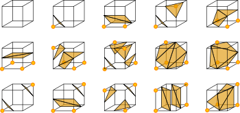
For mesh generation we implemented the marching cubes algorithm from the
marching cubes paper.
We subdivide the entire object space into a multitude of smaller marching cubes.
Then for each marching cube, we take the eight corner points, calculate their isovalues with the iso function and use the returned isovalue to decide if a triangle should be rendered at an edge near that vertex or not.
Then we generate a .obj mesh file containing a list of 3D triangle positions and 3D triangle normal values.
For our implementation, we used a subset of code from
the Polygonize website
that provided: the list of all 256 different triangles we can render, a way to generate an index into the triangle list, and the 3D positions of the triangles.
As part of the mesh generation, we needed to compute the isovalue for each of the voxels (corners of each unit marching cube). Here, we decided to use the density calculation, similar to the one described in fluid-particle generation, to be the isofunction. The isovalue of each voxel is computed by running the isofunction on all the particles within a specific search radius and summing up all the corresponding density.
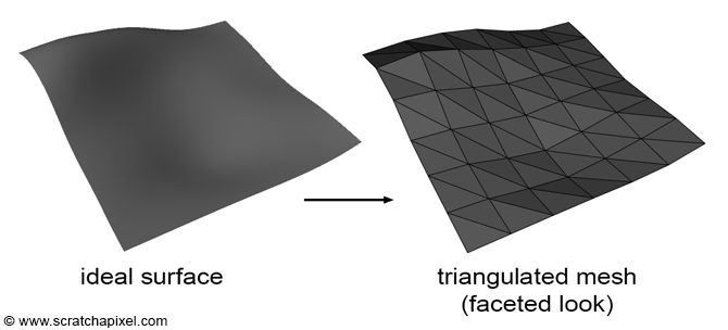
To make the animation look more visually pleasing, we computed the normals for each triangle and cube vertex, or else the animation would look noticeably triangulated. To calculate the normals for each cube vertex, we computed the vector that goes through the vertex and its diagonal vertex counterpart and made that the normal vector. And for the triangle normals we modified the code subset we used to calculate the triangle positions to calculate the triangle normals, with the cube vertex normals as the passed in input.
After running the marching cube algorithm, we are able to generate a list of triangle meshes that represent the surface at each frame.
In order to input our meshes into our rendering software, we need to turn triangle meshes into a .obj file.
In order to do this, we need to write code that will write our triangle vertices, normals, and face definitions into a .obj file.
The code is relatively straightforward: we write the vertices, normal, and face definition line by line into a file.
To import our meshes into blender, we used a third party addon called Stop Motion OBJ to import our OBJ files as a mesh sequence. To make the particle mesh look like water we used a glass BSDF with the same index of refraction as water. To visualize our diffuse particles, we imported them as a .PLY file using the same third party addon. This imported them as points, which we converted to a volume then a mesh.
We wanted to simulate the fluid with a large number of particles to improve the accuracy of the simulation. In order to achieve this high density, we tried to pack a large number of particles in a small box. However, when we tried generating a small box we were having issues with the particles getting launched upwards. We decided to resolve this problem by using a fixed particle density with a larger box and then scaling down the positions of each particle after simulating. By doing this, we are did not experience the blowing-up problem while making the particles denser in our cube.
To run the marching cubes algorithm, we need to find all the particles within a certain distance from each voxel. To do this efficiently, we use the same hashmap as used in the fluid simulation.
To further speed up the program, we store previously calculated isovalues in a map. Since up to 8 cubes can share a single vertex, storing these results allows us to avoid redundant calculations. However, to avoid running out of memory, we throw away results that will no longer be needed.
.ply Files to Render Diffuse Particles
Even though we tried to speed up our marching cubes algorithm as much as possible, it was still too slow to generate a mesh fine enough for diffuse particles.
We tried using OpenVDB to convert the particles to a mesh, but when that did not work, we decided to output the particle positions with .ply files and use Blender's built-in functionality to generate meshes from points.
|
|
|
|
|
|
The main lesson we learned was that tuning parameters is a very important and time consuming process that directly determines the quality of the final output no matter how good the code is. The method we used for tuning parameters for the marching cubes algorithm was trial and error, and for tuning the particle physics simulation parameters, we wrote a Jupyter Notebook script that automated the tuning process, along with plotting the results in Matplotlib to visually verify the quality of the output based on our parameters. Both methods of parameter tuning still took longer than we expected.